Spark Streaming part 1: build data pipelines with Spark Structured Streaming

Spark Structured Streaming is a new engine introduced with Apache Spark 2 used for processing streaming data. It is built on top of the existing Spark SQL engine and the Spark DataFrame. The Structured Streaming engine shares the same API as with the Spark SQL engine and is as easy to use. Spark Structured Streaming models streaming data as an infinite table. Its API allows the execution of long-running SQL queries on a stream abstracted as a table. It is quite easy to use. We based this tutorial on a common workflow where events are consumed from a Kafka topic to familiarize yourself with Spark Structured Streaming and to discover one of the most developer-friendly streaming engines out there.

A brief description of Spark Structured Streaming from its programming guide reads:

Spark Structured Streaming provides fast, scalable, fault-tolerant, end-to-end exactly-once stream processing without the user having to reason about streaming.

This article is the first article of a series of four articles:

• In the first part, a data pipeline with a Spark Structured Streaming application is built.
• The second part concerns the migration of the pipeline to a Hadoop cluster.
• In the third part, the PySpark application was ported to Scala Spark and unit tested.
• The fourth and last part enriches the data pipeline with a Machine Learning clustering algorithm.

This first article focuses on the streaming and present the use case. The streaming data will be ingested with Kafka and then Spark Structured Streaming will be leveraged to process data in near real-time. The second part describes the scenario of the same pipeline on a Hadoop cluster and tackles the difficulties of moving into production.

The Taxi data slightly modified for the Apache Flink Training (edit: original link no longer active, see here) will be used. It contains a collection of ride events with information such as the driver id, the amount paid, and an indication if the ride is starting or ending. Data is available in two compressed files: nycTaxiRides.gz with rides’ essential information including geographical localization, and nycTaxiFares.gz conveying the rides’ financial information. The size of the used dataset is small (below 100MB), but original NYC Taxi Rides data amounts to over 500GB if you wish to run it on a cluster.

The selected use case is the identification of the Manhattan neighborhoods that are most likely to yield high tips. A cab driver with such information could favor places that recently peaked in tips to boost his earning. Note about the pertinence of this dataset, tip data is collected only from payments by card, whereas in reality tips are often given in cash. It’s a scenario entailing the use of streaming processing because the detection of the elevated tip has to be as fast as possible.

Get Kafka and Spark ready

The code below creates a new directory for the project and prepare the environment with both Spark and Kafka installed.

mkdir spark-sstreaming-part1 && cd $_
#Spark 2.4.0 installation
curl http://mirrors.standaloneinstaller.com/apache/spark/spark-2.4.0/spark-2.4.0-bin-hadoop2.7.tgz -o spark-2.4.0-bin-hadoop2.7.tgz
tar xzf spark-2.4.0-bin-hadoop2.7.tgz
ln -sf spark-2.4.0-bin-hadoop2.7 spark
#Kafka 2.2.0 installation
curl https://www-us.apache.org/dist/kafka/2.2.0/kafka_2.12-2.2.0.tgz -o kafka_2.12-2.2.0.tgz
tar xzf kafka_2.12-2.2.0.tgz
ln -sf kafka_2.12-2.2.0 kafka

The streaming results will be printed to the console. Spark’s Driver program output tends to be rich in INFO level logs, which obfuscates the processing results. One acceptable strategy is moving the Spark log level to WARN. It could be done by providing an appropriate “spark/conf/log4j.properties” file. When facing issues, it would be best to reverse to INFO log level.

#Set Spark's console output log level to WARN
cp spark/conf/log4j.properties.template spark/conf/log4j.properties
sed -i -e 's/log4j.rootCategory=INFO/log4j.rootCategory=WARN/g' spark/conf/log4j.properties

A ZooKeeper server and a Kafka broker shall be launched. Also, Kafka topics for each of the Taxi input source have to be created.

kafka/bin/zookeeper-server-start.sh -daemon kafka/config/zookeeper.properties
kafka/bin/kafka-server-start.sh -daemon kafka/config/server.properties
kafka/bin/kafka-topics.sh \
  --create --zookeeper localhost:2181 --replication-factor 1 \
  --partitions 1 --topic taxirides
kafka/bin/kafka-topics.sh \
  --create --zookeeper localhost:2181 --replication-factor 1 \
  --partitions 1 --topic taxifares

Ingestion of the Taxi data into Kafka

In a real-world streaming application, the dataset is unbounded. For the sake of flexibility, this article is based on a finite dataset. It is used to simulate a streaming data flow since data is emitted as on-going events into Kafka. The real world pipeline would work without any modifications in the code. Unix pipes below import the Taxi data into Kafka topics in a one-off fashion.

( curl -s https://training.ververica.com/trainingData/nycTaxiRides.gz \
  | zcat \
  | split -l 10000 --filter="kafka/bin/kafka-console-producer.sh \
    --broker-list localhost:9092 --topic taxirides; sleep 0.2"\
  > /dev/null ) &
( curl -s https://training.ververica.com/trainingData/nycTaxiFares.gz \
  | zcat \
  | split -l 10000 --filter="kafka/bin/kafka-console-producer.sh \
    --broker-list localhost:9092 --topic taxifares; sleep 0.2" \
  > /dev/null ) &

1. A stream is created from a downloaded file without storing anything on the filesystem
2. zcat uncompresses “.gz” file
3. split feeds commands specified by the —filter option into chunks of 10000 messages/events
4. Kafka’s console producer kafka-console-producer.sh publish the messages to the Kafka topic
5. sleep adds 100 milliseconds of delay between each batch of 10000 messages to mimic the sequential nature of a stream
6. Since the kafka-console-producer.sh outputs > characters for each event, > /dev/null redirects the standard output (stdout) to nowhere
7. The & at the very end of the command is added to run everything in the background. It frees the terminal to launch another stream right away

Only two streams of data are simulated in this example. A real-world use case entails multiple streams (e.g. from hundreds of devices in an IoT network) and complex producers.

Kafka’s kafka-console-consumer.sh could be used to verify that data was successfully registered on topics.

kafka/bin/kafka-console-consumer.sh \
  --bootstrap-server localhost:9092 --topic taxirides --from-beginning
kafka/bin/kafka-console-consumer.sh \
  --bootstrap-server localhost:9092 --topic taxifares --from-beginning

This consumer command prints the Kafka stream into the console. Now the data is being collected as expected, the Spark Streaming application can be prepared to consume the taxi rides and fares messages.

Spark Structured Streaming integration with Kafka

Spark Structured Streaming is the new Spark stream processing approach, available from Spark 2.0 and stable from Spark 2.2. Spark Structured Streaming processing engine is built on the Spark SQL engine and both share the same high-level API. The same batch processing code could be used for near real-time stream processing, only the input and output methods need to be modified. The default micro-batch processing model guarantees exactly-once semantics and end-to-end latencies of 100 ms. Since Spark 2.3 there is the experimental continuous processing model allowing end-to-end latencies as low as 1ms with at-least-once guarantees. For the purpose of this article, the default micro-batch approach is sufficient.

The first step is creating a Spark Session and streaming DataFrames subscripted to Kafka’s topics:

from pyspark.sql import SparkSession
spark = SparkSession.builder \
  .appName("Spark Structured Streaming from Kafka") \
  .getOrCreate()

sdfRides = spark \
  .readStream \
  .format("kafka") \
  .option("kafka.bootstrap.servers", "localhost:9092") \
  .option("subscribe", "taxirides") \
  .option("startingOffsets", "latest") \
  .load() \
  .selectExpr("CAST(value AS STRING)") 

sdfFares = spark \
  .readStream \
  .format("kafka") \
  .option("kafka.bootstrap.servers", "localhost:9092") \
  .option("subscribe", "taxifares") \
  .option("startingOffsets", "latest") \
  .load() \
  .selectExpr("CAST(value AS STRING)")

The startingOffsets option is left out to default latest, which obligates us to relaunch the data stream into Kafka when Spark application awaits data. Kafka message has the actual data contained in the “value” column as a string. Before extracting the data from it, the schema has to be prepared. Then, the string in the “value” column is split and used to populate new columns.

from pyspark.sql.types import *

taxiFaresSchema = StructType([ \
  StructField("rideId", LongType()), StructField("taxiId", LongType()), \
  StructField("driverId", LongType()), StructField("startTime", TimestampType()), \
  StructField("paymentType", StringType()), StructField("tip", FloatType()), \
  StructField("tolls", FloatType()), StructField("totalFare", FloatType())])
    
taxiRidesSchema = StructType([ \
  StructField("rideId", LongType()), StructField("isStart", StringType()), \
  StructField("endTime", TimestampType()), StructField("startTime", TimestampType()), \
  StructField("startLon", FloatType()), StructField("startLat", FloatType()), \
  StructField("endLon", FloatType()), StructField("endLat", FloatType()), \
  StructField("passengerCnt", ShortType()), StructField("taxiId", LongType()), \
  StructField("driverId", LongType())])

def parse_data_from_kafka_message(sdf, schema):
  from pyspark.sql.functions import split
  assert sdf.isStreaming == True, "DataFrame doesn't receive streaming data"
  col = split(sdf['value'], ',') #split attributes to nested array in one Column
  #now expand col to multiple top-level columns
  for idx, field in enumerate(schema): 
      sdf = sdf.withColumn(field.name, col.getItem(idx).cast(field.dataType))
  return sdf.select([field.name for field in schema])

sdfRides = parse_data_from_kafka_message(sdfRides, taxiRidesSchema)
sdfFares = parse_data_from_kafka_message(sdfFares, taxiFaresSchema)

Modified sdfRides and sdfFares are ready for processing.

Launching streaming queries in Spark

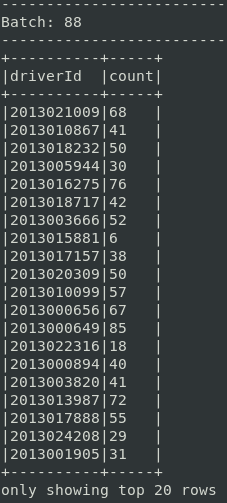
Before developing the target query, let’s verify everything is fine by printing the counts of Taxi rides done by each driver.

query = sdfRides.groupBy("driverId").count()

query.writeStream \
  .outputMode("complete") \
  .format("console") \
  .option("truncate", False) \
  .start() \
  .awaitTermination()

The DataFrame.writeStream interface allows to control output behavior of a streaming DataFrame:

• Spark Structured Streaming supports three output modes: “complete”, “update”, and “append”. Each mode has specific query types they work with. Output modes determine what results (rows from “Result Table”) will be written to the external sink:

  • The outputMode("complete") used above is supported only for aggregation queries. All rows are outputted for every trigger
  • In the outputMode("update"), only new rows and rows changed from the last trigger are outputted
  • In the outputMode("append"), only new rows are outputted to the sink, precisely once. Previous results were already printed and cannot be modified by principle - similarly as it’s impossible to change a file’s existing content by appending a new string. Only queries with each row outputted precisely once (e.g. with select and filter) are supported right away. Queries with aggregates (e.g. with count) entail updating previous results and won’t work in “append” mode unless watermarking and windowing is employed

• There are various sinks available besides format("console") used above. It could be an another Kafka Topic, a file sink, or a memory sink

• A Spark structured streaming query could be started with various triggers that specify time interval before processing a new micro-batch. As the .trigger() option was left out, Spark defaults to processing new data as soon as the previous micro-batch has been processed

The test application is ready to be submitted. In this article, Spark runs in local mode on a single host, while in the next part Spark will run in yarn mode on a Hadoop cluster. The spark-sql-kafka package is obligatory for Spark and Kafka integration. Spark’s application parameters --num-executors, --executor-memory, and --driver-memory are adjusted for a machine with 16GB RAM and could be changed.

spark/bin/spark-submit \
  --master local --driver-memory 4g \
  --num-executors 2 --executor-memory 4g \
  --packages org.apache.spark:spark-sql-kafka-0-10_2.11:2.4.0 \
  sstreaming-spark-out.py

Once the Spark application is up and outputs empty “Batch: 0” with DataFrame headers, it’s time to relaunch the stream of data with the command from Kafka section.

( curl -s https://training.ververica.com/trainingData/nycTaxiRides.gz | zcat \
| split -l 10000 --filter="kafka/bin/kafka-console-producer.sh --broker-list localhost:9092 --topic taxirides; sleep 0.1" > /dev/null ) &

The code developed in this section is available here. Example of the expected output:

Cleaning the Taxi data

A straightforward task is cleaning the data out of all Ride events that either started or ended outside NYC. Also, all “START” events are filtered out because for the purpose of this article only rides that has ended are used (unfinished rides don’t have tip information). It has an advantage of resolving the issue with the Taxi data from Flink tutorial - “endTime” and “startTime” columns of Rides table have switched order for “START” events in respect to “END” events. By keeping only “END” events, only one order is preserved.

LON_EAST, LON_WEST, LAT_NORTH, LAT_SOUTH = -73.7, -74.05, 41.0, 40.5
sdfRides = sdfRides.filter( \
  sdfRides["startLon"].between(LON_WEST, LON_EAST) & \
  sdfRides["startLat"].between(LAT_SOUTH, LAT_NORTH) & \
  sdfRides["endLon"].between(LON_WEST, LON_EAST) & \
  sdfRides["endLat"].between(LAT_SOUTH, LAT_NORTH))
# Notice that rides with faulty geospatial data as e.g. (0, 0) are filtered out also 

sdfRides = sdfRides.filter(sdfRides["isStart"] == "END") #Keep only finished!

The data cleaning step could be developed more. For example, the temporal nature of the data could be leveraged to filter out rides that had negative duration etc. A strategy to clean financial data in sdfFares could be developed as well.

Stream-stream join with Watermarking

From Spark 2.3, Spark Structured Streaming supports stream-stream joins. The goal is to join streaming DataFrames sdfRides and sdfFares. Joined dataset would allow insights from geospatial and financial data considered together. An inner join between two streaming DataFrames is supported only in “append” output mode. Any join could benefit from Watermarking. Watermarking should be considered obligatory for efficient joins.

Watermark defines how much a timestamp can lag behind the maximum event time seen so far. For example, the latest event was at 14h05 and watermark is set to 1 hour. A new event with a timestamp at 13h00 would be dropped while the one at 13h10 would be marked as valid and kept in the Streaming State (buffer). This mechanism limits buffer size for joins and ensures that the dataset won’t grow infinitely. An event isn’t kept forever for a join or an aggregate. Discarding the outdated data also takes care of out-of-order data issues.

The purpose of this join is merging information from two events related to the ride’s end, not joining events corresponding to the start and the end of the Taxi ride. It would make sense to only watermark “endTime” of both DataFrames and define time-constraints only on time difference in ending times. That would be a simple join with small buffer since the difference in ending timestamps shouldn’t be bigger than a few minutes. Unfortunately, the sdfFares DataFrame created from Flink data lacks the “endTime” column and only has the “startTime” column. The ride is payed off at the “endTime” and it would make more sense to have this column available in sdfFares. The join can be done anyways but in a slightly misleading way. The “startTime” has to be used for watermarking of the sdfFares and “endTime” for watermarking of the sdfRides. Consequently, time-constraint relating the beginning and the end of the ride has to be defined for a join.

# Apply watermarks on event-time columns
sdfFaresWithWatermark = sdfFares \
  .selectExpr("rideId AS rideId_fares", "startTime", "totalFare", "tip") \
  .withWatermark("startTime", "30 minutes")  # maximal delay

sdfRidesWithWatermark = sdfRides \
  .selectExpr("rideId", "endTime", "driverId", "taxiId", \
    "startLon", "startLat", "endLon", "endLat") \
  .withWatermark("endTime", "30 minutes") # maximal delay

# Join with event-time constraints
sdf = sdfFaresWithWatermark \
  .join(sdfRidesWithWatermark, \
    expr(""" 
     rideId_fares = rideId AND 
      endTime > startTime AND
      endTime <= startTime + interval 2 hours
      """))

Above, it was defined that no sdfFares nor sdfRides event could be late more than 30 minutes. A Fares event would be kept up to 30 minutes to match it with Ride event, and vice versa. The constraint used on join also specifies that rides longer than 2 hours are dropped.

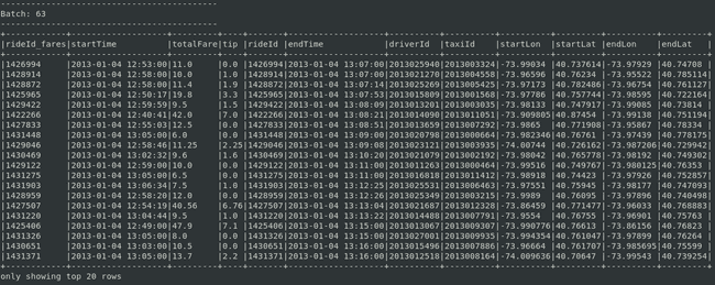
Example micro-batch at this point:

Feature Engineering of neighborhood attribute

Before adding aggregates to streaming, geo points shall be transformed into neighborhoods. This section has little relevance to streaming itself but shows a broadcasting feature available in Spark.

Geographic coordinates of rides could be used to find out which rides have similar routes. A Geo-point has a Manhattan neighborhood assigned in order to approximate position. Such feature creates a partitioning of all rides in Manhattan, useful for grouping. Ride belongs to the given neighborhood if and only if the ride’s “(Lon, Lat)” point is within the neighborhood boundary. This amounts to checking if a point is in a given polygon defined as a collection of points ”[(Lon_A, Lat_A), (Lon_B, Lat_B), …]“.

Zillow data team has prepared Shapefiles with neighborhood boundaries in the largest cities in the U.S. The PyShp Python library is used to read them. The nbhd.jsonl file created below has all Manhattan neighborhoods, one per line. It would be easy to fetch all neighborhoods in NYC, but for the purpose of the article, only Manhattan neighborhoods are considered.

pip install pyshp # if needed
wget https://www.zillowstatic.com/static-neighborhood-boundaries/LATEST/static-neighborhood-boundaries/shp/ZillowNeighborhoods-NY.zip
unzip ZillowNeighborhoods-NY.zip
cat > prep.py <<- EOF
import shapefile
import json
with open('nbhd.jsonl', 'w') as outfile:
  sf = shapefile.Reader("ZillowNeighborhoods-NY")
  shapeRecs = sf.shapeRecords()
  for n in shapeRecs:
    State, County, City, Name, RegionID = n.record[:]
    if City != 'New York' : continue
    if County != 'New York' : continue # New York County corresponds to Manhattan borough
    json.dump({"name":Name, "coord":n.shape.points}, outfile)
    outfile.write('\n')
EOF
python3 prep.py

The even-odd algorithm with the Wikipedia implementation is used way to find out neighborhood to which the geo point belongs:

def isPointInPath(x, y, poly):
  """check if point x, y is in poly
  poly -- a list of tuples [(x, y), (x, y), ...]"""
  num = len(poly)
  i = 0
  j = num - 1
  c = False
  for i in range(num):
    if ((poly[i][1] > y) != (poly[j][1] > y)) and \
        (x < poly[i][0] + (poly[j][0] - poly[i][0]) * (y - poly[i][1]) /
                          (poly[j][1] - poly[i][1])):
      c = not c
    j = i
  return c

Since Spark can use multi-line JSON file as a data source, all the polygons can be load into the DataFrame with spark.read.json(). Each time an executor on a Worker Node processes a micro-batch, a separate copy of this DataFrame would be sent. Knowing the lookup data is not changing and tasks across multiple stages need the same data, sending it repeatedly isn’t the best solution. Instead, Spark’s broadcasting feature could be used. A small lookup static variable containing neighborhoods’ polygons shall be stored in the read-only in-memory cache of all nodes. An explicit broadcast variable could be defined with SparkContext.broadcast() method provided with a key-value dictionary.

nbhds_df = spark.read.json("nbhd.jsonl") #easy loading data
lookupdict = nbhds_df.select("name","coord").rdd.collectAsMap() # cast the DataFrame
broadcastVar = spark.sparkContext.broadcast(lookupdict) #use broadcastVar.value from now on

Broadcasting the neighborhoods enables access to the lookup table from any user-defined function (UDF). A neighborhood could be assigned to each ride in a DataFrame’s column with the UDF defined below.

#Approx manhattan bbox 
manhattan_bbox = [[-74.0489866963,40.681530375],[-73.8265135518,40.681530375], \
[-73.8265135518,40.9548628598],[-74.0489866963,40.9548628598],[-74.0489866963,40.681530375]]

from pyspark.sql.functions import udf
def find_nbhd(lon, lat):
  '''takes geo point as lon, lat floats and returns name of neighborhood it belongs to
  needs broadcastVar available'''
  if not isPointInPath(lon, lat, manhattan_bbox) : return "Other"
  for name, coord in broadcastVar.value.items():
    if isPointInPath(lon, lat, coord):
      return str(name) #cast unicode->str
  return "Other" #geo-point not in neighborhoods

find_nbhd_udf = udf(find_nbhd, StringType())
sdf = sdf.withColumn("stopNbhd", find_nbhd_udf("endLon", "endLat"))
sdf = sdf.withColumn("startNbhd", find_nbhd_udf("startLon", "startLat"))

Example of expected output at this stage:

The Taxi data is now prepared to answer questions based on Manhattan neighborhoods and financial data. It’s possible to answer the following question:

What Manhattan neighborhoods should Taxi driver choose to get a high tip?

Adding aggregation

The final operation is averaging over the “tip” column, grouped by ending neighborhoods and 30 minutes windowing (updated in 10-minute intervals). It would be preferable to run 2 hours windows with triggers every minute, but that would demand high computing resources.

tips = sdf \
  .groupBy(
    window("endTime", "30 minutes", "10 minutes"),
    "stopNbhd") \
  .agg(avg("tip"))

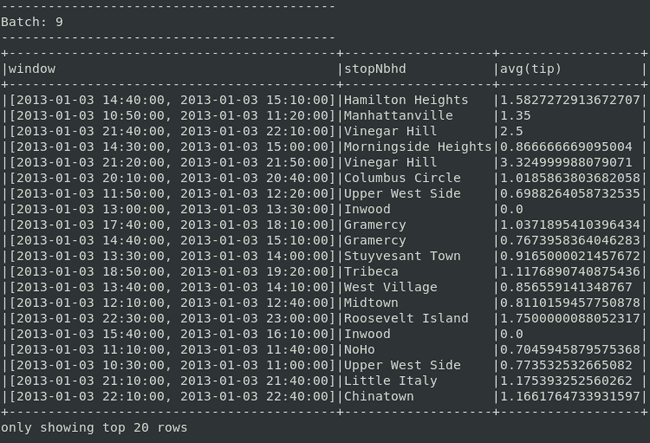
The complete code is available here in single file. An example of the final results is below.

Based only on top 20 rows, a driver would receive a notification at 21h50 that going to Vinegar Hill for a next ride is a good idea

Few empty batches in the beginning are acceptable. It’s expected behavior for the “append” output mode, as the engine starts outputting results only after the initial watermark has passed. It would be useful to sort results by timestamps or according to tips. Unfortunately, sorting operations are not yet supported on streaming DataFrames in “append” mode. It’s Spark Structured Streaming limitation which may be addressed in the future.

Future work

• This tutorial run local and not on a Big Data infrastructure for distributed processing. The purpose of the second part is placing the same processing in a production environment with Spark on YARN
• The article was intended to focus on streaming, at the cost of other aspects. For example, the approach for obtaining neighborhoods is brute and non-scalable. Only Manhattan neighborhoods were considered, but with efficient Geospatial data treatment, it would be possible to consider all NYC neighborhoods
• Used neighborhoods are administrative boundaries, which is an artificial grouping. Making use of Machine Learning algorithm for clustering could provide more useful grouping than neighborhoods

Summary

Spark Structured Streaming was used extensively to develop a streaming data pipeline. After ingestion of data from Kafka, Taxi rides were processed in near real-time in Spark. The stream-stream join was performed, as well as a simple aggregation operation. A simple feature engineering step was also taken in order to fulfill the use case. The biggest drawback of the project presented in the article is the lack of Big Data infrastructure. All work has been done on a local machine. The goal of the next part in this two-part series shall be transferring the processing into a Hadoop cluster.