Optimization of Spark applications in Hadoop YARN

Apache Spark is an in-memory data processing tool widely used in companies to deal with Big Data issues. Running a Spark application in production requires user-defined resources. This article presents several Spark concepts to optimize the use of the engine, both in the writing of the code and in the selection of execution parameters. These concepts will be illustrated through a use case with a focus on best practices for allocating ressources of a Spark applications in a Hadoop Yarn environment.

Spark Cluster: terminologies and modes

Deploying a Spark application in a YARN cluster requires an understanding of the “master-slave” model as well as the operation of several components: the Cluster Manager, the Spark Driver, the Spark Executors and the Edge Node concept.

The “master-slave” model defines two types of entities: the master controls and centralizes the communications of the slaves. It is a model that is often applied in the implementation of clusters and/or for parallel processing. It is also the model used by Spark applications.

The Cluster Manager maintains the physical machines on which the Driver and its Executors are going to run and allocates the requested resources to the users. Spark supports 4 Cluster Managers: Apache YARN, Mesos, Standalone and, recently, Kubernetes. We will focus on YARN.

The Spark Driver is the entity that manages the execution of the Spark application (the master), each application is associated with a Driver. Its role is to interpret the application’s code to transform it into a sequence of tasks and to maintain all the states and tasks of the Executors.

The Spark Executors are the entities responsible for performing the tasks assigned to them by the Driver (the slaves). They will read these tasks, execute them and return their states (Success/Fail) and results. The Executors are linked to only one application at a time.

The Edge Node is a physical/virtual machine where users will connect to instantiate their Spark applications. It serves as an interface between the cluster and the outside world. It is a comfort zone where components are pre-installed and most importantly, pre-configured.

Execution modes

There are different ways to deploy a Spark application:

The Cluster mode: This is the most common, the user sends a JAR file or a Python script to the Cluster Manager. The latter will instantiate a Driver and Executors on the different nodes of the cluster. The CM is responsible for all processes related to the Spark application. We will use it to handle our example: it facilitates the allocation of resources and releases them as soon as the application is finished.
The Client mode: Almost identical to cluster mode with the difference that the driver is instantiated on the machine where the job is submitted, i.e. outside the cluster. It is often used for program development because the logs are directly displayed in the current terminal, and the instance of the driver is linked to the user’s session. This mode is not recommended in production because the Edge Node can quickly reach saturation in terms of resources and the Edge Node is a SPOF (Single Point Of Failure).
The Local mode: the Driver and Executors run on the machine on which the user is logged in. It is only recommended for the purpose of testing an application in a local environment or for executing unit tests.

The number of Executors and their respective resources are provided directly in the spark-submit command, or via the configuration properties injected at the creation of the SparkSession object. Once the Executors are created, they will communicate with the Driver, which will distribute the processing tasks.

Resources

A Spark application works as follows: data is stored in memory, and the CPUs are responsible for performing the tasks of an application. The application is therefore constrained by the resources used, including memory and CPUs, which are defined for the Driver and Executors.

Spark applications can generally be divided into two types:

Memory-intensive: Applications involving massive joins or HashMap processing. These operations are expensive in terms of memory.
CPU-intensive: All applications involving sorting operations or searching for particular data. These types of jobs become intensive depending on the frequency of these operations.

Some applications are both memory intensive and CPU intensive: some models of Machine Learning, for example, require a large number of computationally intensive operation loops and store the intermediate results in memory.

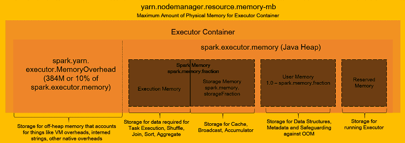
The operation of the Executor memory has two main parts concerning storage and execution. Thanks to the Unified Memory Manager mechanism, memory-storage and run-time memory share the same space, allowing one to occupy the unused resources of the other.

The first is for storing data in the cache when using, for example, .cache() or broadcast().
The other part (execution) is used to store the temporary results of shuffle, join, aggregation, etc. processes.

Memory allocation to Executors is closely related to CPU allocation: one core performs a task on one partition, so if an Executor has 4 cores, it must have the capacity to store all 4 partitions as well as intermediate results, metadata, etc… Thus, the user has to fix the amount of memory and cores allocated to each Executor according to the application he wants to process and the source file: a file is partitioned by default according to the total number of cores in the cluster.

This link lists various best practices for cluster use and configuration. The following diagram, taken from the previous link, gives an overview of how the memory of an Executor works. An important note is that the memory allocated to an Executor will always be higher than the specified value due to the memoryOverhead which defaults to 10% of the specified value.

How a Spark Application Works

In a multi-user cluster, the resources available to each user are not unlimited. They are constrained to a given amount of memory, CPU and storage space, in order to avoid monopolization of resources by a limited number of users. These allocation rules are defined and managed by the cluster administrator in charge of its operation.

In the case of Apache YARN, these resources can be allocated by file. This means that a user may only be allowed to submit applications in a single YARN queue in which the amount of resources available is constrained by a maximum memory and CPU size.

The components and their resources used by a Spark application are configurable via:

the spark-submit command using the arguments --executor-memory, --executor-cores, --num-executors, --driver-cores and --driver-memory arguments.
the SparkSession object by configuring, for example, .config("spark.executor.instances", "7") (see the scripts in the GitHub project).
the options in the spark-defaults.conf configuration file.

The user can also let the Spark decide how many Executors are needed depending on the processing to be done via the following parameters:

spark = SparkSession.builder \
    .appName("<XxXxX>") \
    .config("spark.dynamicAllocation.enabled", "true") \
    .config("spark.executor.cores", "2") \
    .config("spark.dynamicAllocation.minExecutors", "1") \
    .config("spark.dynamicAllocation.maxExecutors", "5") \
    .getOrCreate()

Thus, the application does not monopolize more resources than necessary in a multi-user environment. More details are described in this article explaining how Facebook adjusts Apache Spark for large-scale workloads.

Regarding the underlying filesystem where data is stored, two optimization rules are important:

Partition size should be at least 128MB and, if possible, based on a key attribute.
The number of CPUs/Executor should be between 4 and 6.

In the Spark application presented below, we will use the 2018 New York Green Taxi dataset. The following script will download the file and save it in HDFS:

# Download the dataset
curl https://data.cityofnewyork.us/api/views/w7fs-fd9i/rows.csv?accessType=DOWNLOAD \
  -o ~/trip_taxi_green2018.csv
# Create a HDFS directory
hdfs dfs -mkdir ~/nyctrip
# Load the dataset into HDFS
hdfs dfs -put \
  ~/trip_taxi_green2018.csv \
  ~/nyctrip/trip_taxi_green2018.csv \
  -D dfs.block.size=128M
# Remove the original dataset
rm ~/trip_taxi_green2018.csv

Our file of 793MB divided into 128MB blocks gives us 793/128 = 6.19 or 7 partitions.

If we ask for 7 Executors, they will have respectively in memory ~113MB. With 4 Executors with 2 CPUs, this time they will have ~200MB of data. We have to think about the memory allocation according to the processed application: if the dataset is transformed several times, a good starting point is to allocate twice as many GB of RAM as there are cores per Executors.

Developing and processing a Spark application

We will discuss several aspects of optimization by writing a simple Spark application in Python. This will be deployed in Spark via YARN using the cluster deployment mode. As stated above, we will use the data from the 2018 New York green taxis. The problem will be to determine which of the two taxi companies referenced in the dataset was the most efficient in terms of trip numbers processed in 2018.

In this part, we detail each part of the code. The complete scripts are available on GitHub.

Importing and declaring a SparkSession

For the sake of clarity, imports of Spark classes and functions are generally reported first. In one Spark application, we explained that the user must declare a SparkSession' followed by the builder’ class in order to name and configure the processing options of the application via appName() and config("key", "value"). The .getOrCreate() argument checks whether a SparkSession already exists or creates a new one. If a SparkSession already exists and a new one is created, the options for the new one will also be added to the previous one.

from pyspark.sql import SparkSession
from pyspark.sql.functions import desc, broadcast
spark = SparkSession.builder \
    .appName ("Best Driver 2018") \
    .config("spark.sql.shuffle.partitions", "7") \
    .config("spark.executor.memory", "2g") \
    .config("spark.executor.instances", "4") \
    .config("spark.executor.cores", "2") \
    .getOrCreate()

Importing the dataset

When a Spark application is processed in Batch processing, the user has the choice of declaring the schema of the dataset or letting Spark infer this schema. This is not the case for streaming applications where the user has to declare the schema. Declaring the data schema can be done via a DDL format (which is used here) or via the use of the StructType and StructField types.

schema = "VendorID INT,pickup_datetime TIMESTAMP,dropoff_datetime TIMESTAMP,store_and_fwd_flag STRING,RatecodeID INT,PULocationID INT,DOLocationID INT,passenger_count INT,trip_distance FLOAT,fare_amount FLOAT,extra FLOAT,mta_tax FLOAT,tip_amount FLOAT,tolls_amount FLOAT,ehail_fee FLOAT,improvement_surcharge FLOAT,total_amount FLOAT,payment_type INT,trip_type INT,congestion_surcharge FLOAT"

driver_df = spark.read \
.csv(path="/home/ferdinand.de-baecque-dsti/nyctrip/trip_taxi.csv", schema=schema,header=True) \
# .csv(path="/home/ferdinand.de-baecque-dsti/nyctrip/trip_taxi.csv", inferSchema=True,header=True) \
.select("VendorID") \
.repartition(7, "VendorID")

Here we use the .csv() function which is part of the DataFrameReader class and allows to configure several parameters to create a DataFrame from the dataset. Spark partitions the data according to the total number of cores in the cluster. We end up “repartitioning” the DataFrame according to the VendorID attribute using the .repartition(<#_partitions>, <"column_name">) function.

Reading without schema: with the option inferSchema=True.

Reading with schema: with the schema=schema option.

Reading the dataset is faster when the user declares his schema.

Finally, if we remove the .select("VendorID") part from driver_df, we have:

Request definition

The query of our problem is in one line thanks to the native Spark functions called higher-ordered functions. They are optimized by the engine and are to be preferred to User-Defined Functions (UDF) written by a user. Using a higher-order function allows Spark to understand what the user is trying to achieve and optimize the processing of the application. On the other hand, Spark does not see the content of a UDF (opaque) and therefore, does not understand the purpose of the UDF and is not able to optimize its processing. New native functions are added as Spark evolves.

Native functions work as follows: the engine builds several “logical” planes and then implements and compares the way these planes are processed to select the best one - it is this plane, called Physical Plan, which is printed with the .explain() function. These optimization aspects are related to the Tungsten Project and the Catalyst Optimizer.

count_trip = driver_df.groupBy("VendorID").count().sort(desc("count"))
count_trip.explain()
count_trip.show()

In our query, we start by grouping the companies together with groupBy(). Then we count the number of occurrences with count(). Finally, we sort the results with sort(desc()) so that the best performing company appears at the top. This last function is part of the family of wide transformations creating a shuffle between Executors passing through the network; the graph below illustrates this concept. By default, Spark creates 200 partitions when these wide transformations are called; a good practice is to redefine this value according to the scenario.

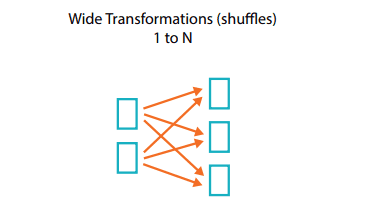
When declaring the SparkSession class, we set .config("spark.sql.shuffle.partitions", "7"). This option is related to wide transformations, it limits the creation of partitions after a shuffle: the sort(desc()) operation creates 7 partitions instead of 200.

Without this configuration option, we have:

With the option, we have:

Changing the default value of this configuration parameter can greatly optimize these types of transformations. Here, we go from 0.6 to 0.2 seconds, limiting the number of partitions created by the shuffles to 7. The value has been set according to the number of cores in the cluster.

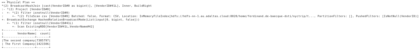
The physical plane given by explain() is:

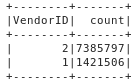
Finally, .show() is an Action in Spark which returns the result in the logs or in the console depending on Spark’s configuration. It is this function that will trigger the execution of the transformations that precede it in the application. This is the principle of Lazy Evaluation.

The result of our query is:

Processing the request

The previous captures were made with 7 Executives of 1 CPU and 2GB of RAM. The command to run the application in Spark is:

spark-submit --master yarn --deploy-mode cluster \
  --queue adaltas ./scripts_countTrip/query_7Exécuteurs.py

In the SparkSession.builder, if we set to 4 Executives each having 2 CPUs and 4g of RAM while modifying spark.shuffle.partitions with 8, we get a gain of 1 second on the scan of our file:

spark-submit --master yarn --deploy-mode cluster \
  --queue adaltas scripts/scripts_countTrip/query_4executors.py \
  <Path_to_your_HDFS_Local_file_>

The documentation advises to have 2-3 times more partitions than cores available in the cluster, the data and thus, the tasks will be better distributed. Cores do not necessarily process a job at the same speed. For example, we can repartition our file into two partitions according to the VendorID column (because it has two occurrences) by adding the .repartition(2, "VendorID") function at the end of driver_df. With 2 Executors with 1 CPU, one CPU will process its .count() much slower than the other.

Joins in Spark

Joining operations are recurrent in Spark applications, they must be optimized to avoid unnecessary shuffles. We will create a small dataset directly in the application and the goal will be to join this small DataFrame with our large taxi database. In this case, a good practice is to use the broadcast() function to duplicate the contents of the small DataFrame on all Executors. Shuffles will not be necessary because each Executor will have its own partition of the large DataFrame and also the entire small DataFrame.

Join 1: Default join.

littleDf = spark.createDataFrame( 1, "The First Company"), (2, "The second company"), ("VendorID", "VendorName")
# Join 1
detailledDf = driver_df.join(littleDf, driver_df["VendorID"] == littleDf["VendorID"])
detailedDf.explain()
detailedDf.show()

spark-submit --master yarn --deploy-mode cluster --queue adaltas --
  scripts/scripts_join/default_join.py \
  <Path_to_your_HDFS_Local_file_>

The Physical Plan is:

The execution time of the application is:

Join 2: Using the BroadcastJoin.

detailledDfBroad = driver_df.join(broadcast(littleDf), driver_df["VendorID"] == littleDf["VendorID"])
detailedDfBroad.explain()
detailedDfBroad.show()

spark-submit --master yarn --deploy-mode cluster --queue adaltas --
  scripts/scripts_join/broadcast_join.py \
  <Path_to_your_HDFS_Local_file_>

The Physical Plan gives:

The execution time:

The broadcast() technique takes us from ~13 seconds to ~10 seconds in total. This is effective if the entire small dataset can be stored in the cache of each Executors.

Finally, doing what the Spark documentation recommends and knowing the number of blocks in HDFS - that is, spreading the data over 16 (8CPUx2) partitions and setting the shuffles to 16 partitions - reduces the total TaskTime of the join 2 by 0.1 seconds:

spark-submit --master yarn --deploy-mode cluster --queue adaltas scripts_join/final_countJoin.py

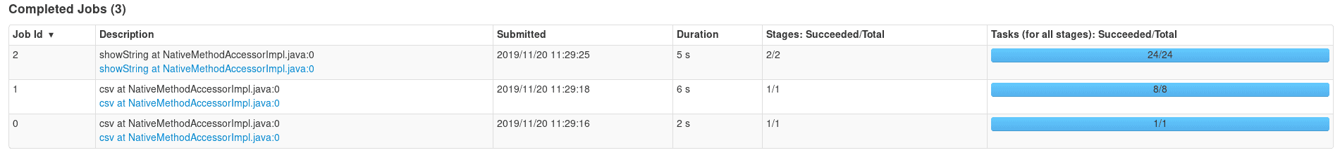
Monitoring

All screenshots for the application come from the YARN ResourceManager web interface. This is where all the information from the Spark applications can be found. Thanks to the Spark History Server which is activated in the cluster, the metrics of the Spark applications are accessible after their processing.

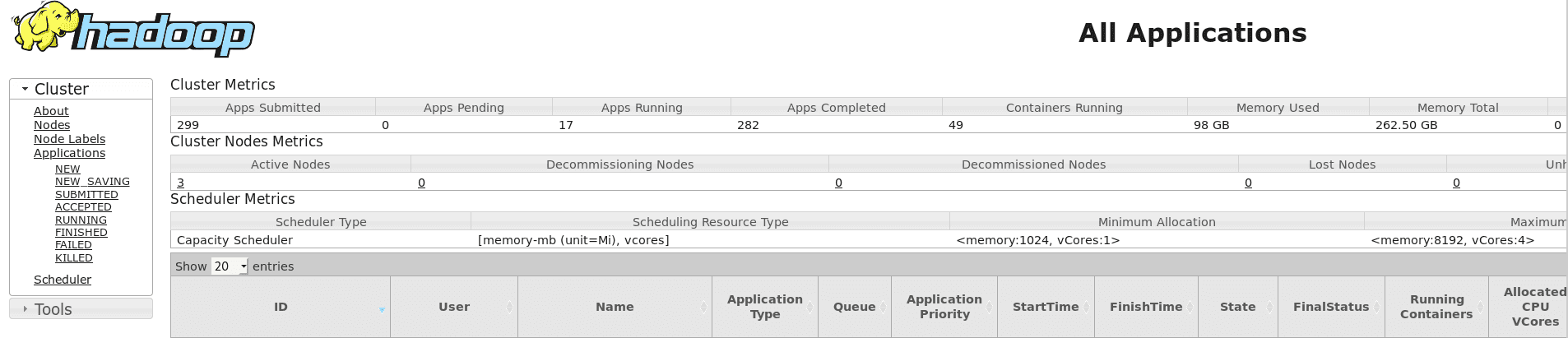
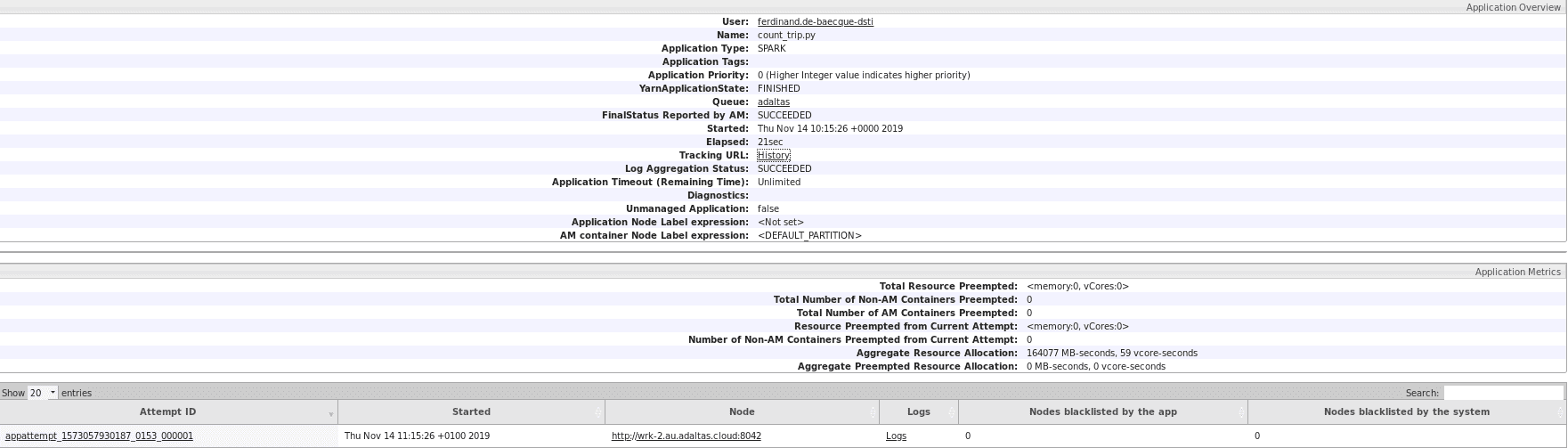
By clicking on the application ID: you can either look at its Logs - where the query results appear in my case - or click on ApplicationMaster / History to get details about its tasks and Executors.

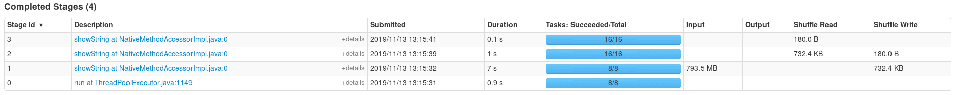
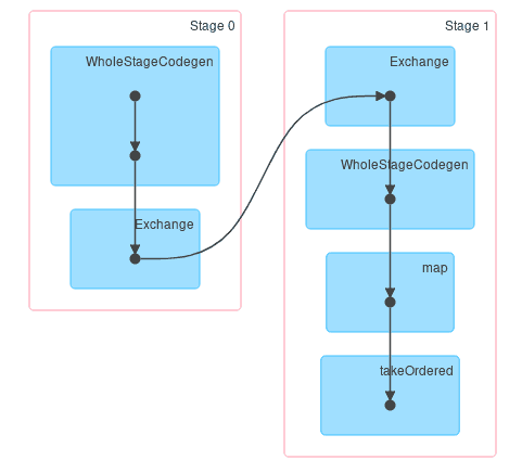
After clicking on History and going to the Stages tab, you can see the DAG (Direct Acyclic Graph) of each stages which is equivalent to a part of the content returned by explain() in graphical form:

If a Spark user wants to standardize the Task Time of each Executor as proof of the correct distribution of data, this information can be found in the Executors tab:

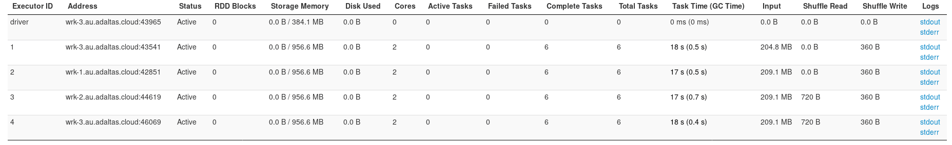
If this is not the case, there is often a problem with the distribution of the dataset. One solution is to increase the number of partitions using the .repartition() function, or partition the dataset before consuming it in Spark. If your application is taking longer than you thought, you can track the progress of each Executor’s tasks by going to the Executors tab and clicking on the different Thread Dumps.

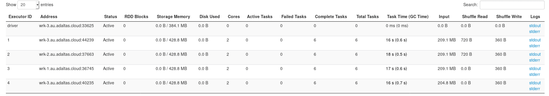
Here, reducing the RAM of the Executors to 1GB instead of 2 has no impact: no transformation is done on all the data. This choice is specific to the scenario because each Executor has 2 partitions with a total of ~200MB. This excess memory can be used by another application.

Conclusion

A number of applications run concurrently in a production environment: the proper allocation of resources to Spark components tends to maximize the performance of an application as well as the number of applications hosted.

We have presented, through a use case, the relationships between cores & partitions, memory & transformations as well as the operation of native functions. Our application was written in Python although this language adds a step to the processing, called SerDe, which this article explains very well. This is the main reason why applications written in Scala perform better. Although it is not our case here, a comparison is made in GitHub. As far as data consumption is concerned, Spark advises to use the Parquet format: it keeps the data schema, the data is compressed and saved by columns (attributes) which makes it easier to extract.

Share this article