H2O in practice: a protocol combining AutoML with traditional modeling approaches

H20 comes with a lot of functionalities. The second part of the series H2O in practice proposes a protocol to combine AutoML modeling with traditional modeling and optimization approach. The objective is the definition of workflow we could apply to new use cases to gain performance and delivery time.

In partnership with EDF Lab and ENEDIS, our common goal is to estimate the difficulty to onboard with the H2O platform, to understand how it works, and to find its strengths and weaknesses in the context of a real-life project.

In the first article, a real-life experience with H2O, the challenge was to build a model with the help of AutoML, and compare it with a reference model, built with a traditional approach. For the second challenge, we were given a ready-to-use dataset from a different business problem (still related to the preventive maintenance) and five days to produce the best model with H2O. To prepare for it, we devised an operational protocol, which we present in this article. It helped us to train a baseline model comparable to the existing one in only two days.

This protocol provides guidance on how to combine AutoML modeling with individual model algorithms for increased performance. The duration of training is analyzed across two examples to get a global picture of what to expect.

Environment, datasets and project descriptions

Project 1, the detection of segments of low-tension underground cables in the need of replacement: train and test set had a bit over 1 million rows and 434 columns each. For this use case, we were using Sparkling Water, which combines H2O and Spark and which distributes the load across a Spark cluster.

• H2O_cluster_version: 3.30.0.3
• H2O_cluster_total_nodes: 10
• H2O_cluster_free_memory: 88.9 Gb
• H2O_cluster_allowed_cores: 50
• H2O_API_Extensions: XGBoost, Algos, Amazon S3, Sparkling Water REST API Extensions, AutoML, Core V3, TargetEncoder, Core V4
• Python_version: 3.6.10 final

Project 2, preventive maintenance, confidential: train and test set had about 85.000 rows each. 605 columns were used for training. For this case, we were using a non-distributed version of H2O, running on a single node.

• H2O_cluster_version: 3.30.1.2
• H2O_cluster_total_nodes: 1
• H2O_cluster_free_memory: 21.24 Gb
• H2O_cluster_allowed_cores: 144
• H2O_API_Extensions: Amazon S3, XGBoost, Algos, AutoML, Core V3, TargetEncoder, Core V4
• Python_version: 3.5.2 final

In both cases, the task was a classification of a heavily unbalanced dataset (< 0.5% of class 1). AUCPR was used as an optimization metric during training. As the final model evaluation, two business metrics were calculated, both representing the number of failures on two different cumulative lengths of feeders. 5-fold cross-validation was used to validate the models. The challenge in both projects was to compare the best model from H2O with the reference in-house model, which was already optimized.

Protocol for modeling with H2O

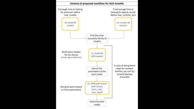
We combined AutoML functionalities with individual modeling algorithms to get the best of both worlds. After trying different approaches, we found the proposed protocol the most concise and straightforward.

1. Depending on the time available:

• If you have enough time, run AutoML to construct many models (30+) without the time limit, to get the longest and the most accurate training (H2OAutoML: max_models).
• If you lack time, or if you are looking only for an approximate result to estimate the baseline performance, define the maximal time of training (H2OAutoML: max_runtime_secs).

2. Calculate a business metric (and/or the additional metrics) for each model and collect them in a custom-defined leaderboard.

3. Merge AutoML leaderboard and a custom-defined leaderboard and inspect:

• Which family of models reaches the highest score?
• How do business and statistical metrics correlate?
• Are any models performing so badly that we don’t want to spend additional time optimizing them?

Due to the confidentiality of the project, we will only describe the results to illustrate the example. The XGBoost family performed much better than any other algorithm. Deep learning performed the worst, which is not surprising on tabular data. For instance, the best XGBoost model found 3-4x more incidents than the best deep learning model, depending on the business metric. The second most performant family was GBM, which in the best case found about 90 % of the incidents of XGBoost. In both projects, the models with the highest AUCPR had the highest business metrics, but generally, the correlation was not great.

4. Run an AutoML grid search on the most successful families of algorithms (H2OAutoML: include_algos). Test many models. Select the models which you want to optimize (models of interest) and save them.

5. Print out the actual parameters of the models of interest (h2o.get_model(model_name).actual_params).

6. Use those parameters as a base in the manual definition of the model. Define the hyperparameters for grid search (H2OGridSearch). If you want to test many or if you lack time, use the random grid search strategy. Otherwise, build the models from all the combinations of the hyperparameters (cartesian strategy).

7. Compute additional metrics on grid search models and optionally inspect the variable importance. The models with similar scores can be based on a different set of variables, which might be more important for the business context than just the score.

8. Select the best model(s) for each family and save it.

9. Optionally, build stacked ensembles and recalculate the additional metrics.

How long does it take?

We were using two datasets of different sizes (1 million rows x 343 columns and 85.000 rows x 605 columns). Since they were processed in two different environments, we cannot compare the processing times directly. With the rough estimates of the duration of each phase, we would like to give you an idea of what you can expect.

Workflow in the Project 1:

• build 40 AutoML models → ~ 8.5 h
• extract the parameters of the best model of each family and define the hyperparameters for optimization (in this case, XGB and GBM)
  • random search:
    • 56 XGB models → ~ 8 h (+ business metrics → ~ 4.5 h)
    • 6 GBM models → ~ 1 h (+ business metrics → ~ 0.5 h)
• save the best models

Considering that the dataset was not very large (< 200 MB), we were surprised that it took so long for AutoML to finish 40 models. Maybe they didn’t converge well, or we should optimize the cluster resources. Our preferred solution was to start the long computations at the end of the day and have the results in the morning.

Workflow in the Project 2:

• run AutoML for 10 min (fixed time; + business metrics ~ 15 minutes)
• build 30 GBM models with AutoML → ~ 0.5 h (+ business metrics → ~ 1 h)
• extract the parameters of the best model and define the hyperparameters for grid search
• random search: 72 GBM models → ~ 1 h (+ business metrics → ~ 2 h)
• save the best model

The second dataset was rather small, and we manage to execute all the steps within one working day.

How good were the models?

The comparison was based solely on the values of the business metrics. We didn’t perform any proper statistical tests on the results, although we took into account the variance of our results. Thus, it’s not to be taken as a benchmark but as an observation. In both cases, we managed to produce the models with roughly the same performance as the references. Usually, we had several candidates with similar scores. Most importantly, we achieved this in only a fraction of the time needed for the reference model.

Conclusion

We showed on two real-life problems how to shorten the time to build a good baseline model by leveraging automated machine learning with H2O. After we invested time in understanding the advantages and the limitations of the platform, we were able to build a model comparable to the reference model in just a couple of days. This is a significant speed-up over the traditional approach. Next to that, user-friendly API shortens the coding time and simplifies the maintenance of the code.

Acknowledgements

The collaborators who contributed to this work are:

• Somsakun Maneerat, EDF Lab, Data scientist
• Benoît Grossin, EDF Lab, Project manager
• Jérémie Mérigeault, ENEDIS, Data scientist